Dairy Trading Strategies: Mean Reversion, Long-Run Mean & Half-life

Insight Focus

• Assets tend to revert to their average price over time.
• We can use statistics to confirm mean reversion potential in dairy.
• We look at long-run mean, half-life, and timing.

Definition of mean reversion: Mean reversion is a financial term for the assumption that an asset’s price will tend to converge to the average price over time.

Definition of half-life: the time required for a quantity (of substance) to reduce to half of its initial value.

Definition of volatility: a statistical measure of the dispersion of returns for a given security or market index.

Exploring Mean Reversion:

• I first touched on this concept with a dairy context on Czapp back in 2020.
• Mean reversion is a theory that a product has a long-term average price (often called the “Long Run Mean” or “LRM” for short) and that its price at a given point in time will tend toward that LRM.
• Think of the LRM as a magnet that gets stronger the further the price gets away from it. For example, if the LRM of a product is calculated to be $100 USD/MT and the product is currently trading at a price of $70 USD/MT then theory of mean reversion is that in the absence of other influences, the price should tend upward toward its LRM.
• Another way of conceptualizing a mean reversion strategy is that it is like a cross-commodity spread trade between one product and itself.

Testing Mean Reversion:

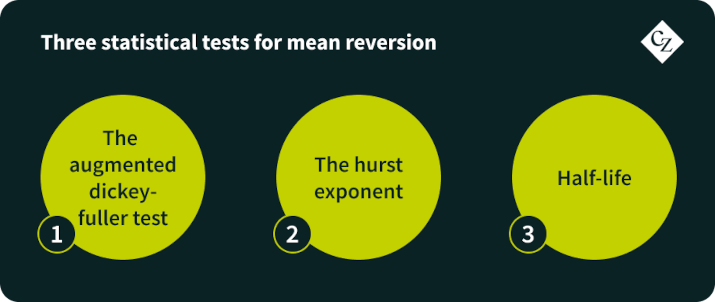
• There are statistical tests that an analyst can do to give them confidence that the commodity which they are investigating is mean-reverting. Three key concepts are the Augmented Dickey-Fuller test, the Hurst exponent and half-life.
• The ADF test helps to determine whether a time series has a unit root or is stationary (mean-reverting). If a unit root is found then the commodity can be said to have a “drift” i.e. a changing mean or variance as time goes on, and not be mean-reverting.
• The Hurst exponent attempts to quantify the persistence of a time series over a range of time scales, essentially measuring the strength of the “long-term memory” of a time series. A value of <0.5 indicates that a commodity is mean reverting (>0.5 is trending).
• Half-life estimates how long it takes for a time series to return halfway to its mean after a deviation. A shorter half-life indicates stronger mean reversion characteristics.

Trading with Mean Reversion:

• Once you are confident that your commodity does exhibit mean reversion, the next step is to calculate its LRM and assess where current pricing is on the statistical distribution relative to that LRM.
• If your commodity is “far” from the LRM at present then there may be a trading opportunity.

Non-technical readers can skip to the case study without any loss in understanding.

• Take your time-series of price data for the commodity under review. I am using daily SGX-NZX WMP pricing here. For mean-reversion analysis I prefer to use log price data as this stabilizes the variance and improves the likelihood of stationarity which is important in a mean reversion context.
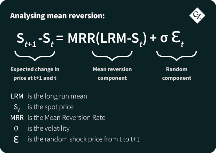
• We can then estimate the Mean Reversion Rate (“MRR”), α above, by regressing price changes against price. The slope of the regression line can be interpreted as a measure of how quickly prices tend to move back toward their historical average after experiencing a deviation. MRR is the negative of the slope in this regression. We take the negative of the slope of the regression line because doing so indicates that as the change in price increases (either positive or negative), the subsequent change in the opposite direction becomes more likely i.e. it captures this reversion behavior.
• Given the dynamic nature of markets it might be useful to conduct this regression on a shorter window of data than that of your whole time series. This can then enable interesting observations of MRR developing over time.
• The spot observation of MRR can be quite volatile and susceptible to market movements. I like to take an exponentially weighted moving average of the MRR to smooth this effect out. This has the benefit of including past observations while weighting more on what has happened to the MRR more recently.
• With the MRR now known you can calculate two important other values: the long-run mean (“LRM”) and the half-life.
• To calculate the LRM you divide the intercept of the regression by the MRR. Remember if you have been using log data to take an exponential of the result of this calculation to get it back into outright price terms.
• A note on the LRM calculation: Dividing the intercept by the mean reversion rate provides a measure of the magnitude of reversion relative to the speed of reversion. This calculation gives you a price value for the expected LRM now when the change in price is zero.
• You can then calculate the half-life of the commodity under observation as follows: Half-life = (ln(2)) / Mean Reversion Rate

Case Study using SGX-NZX WMP data and Trading Insight:

• Values below are as at 24th August, 2023:
  • a) Spot price = $2,460 USD/MT
  • b) MRR = -0.016, this means the WMP price is expected to revert by 1.6% or approx. $40 USD/MT per working day toward its equilibrium level.
  • c) LRM = $3,700 USD/MT
  • d) Half-life = 43.3 working days, this means that in the absence of any other market shocks we would expect that the spot price should be halfway back towards the LRM (i.e. $3,080 USD/MT) by the 24th of October 2023.
  • e) Volatility = 15.9%. The next article in the series will specifically address volatility, its calculation and trading strategies around this. For this article please just take this as given.
• In the absence of any other current or expected market dynamics, in the above example a trader would be interested to buy WMP.
• The relevant SGX-NZX WMP futures for one half-life would be November 2023 and these are currently trading at $2,650 USD/MT. The trader would buy these futures believing them to be mispriced by $430 USD/MT and seek to profit from these futures increasing in price as the spot price is pulled up toward the LRM.

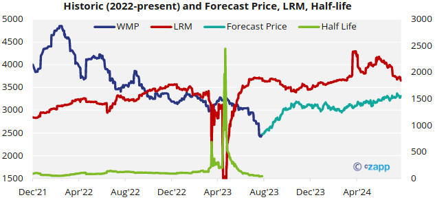
• The above chart may appear messy but it can help conceptualize mean-reversion well.
  • a) The red line is the calculated LRM over time. Where this becomes volatile during May-23 the output is non-sensical but we can take this to be a period where a new LRM is being informed. From mind-June a new LRM is established in the $3500-3700 range.
  • b) Prior to the new LRM being informed, half-life had been stable around 100 days. It is interesting to note that the modeled value from June 2023 is shorter at around 45 days based on faster mean reversion.
  • c) We can use the values here and the equation above to simulate a potential set of prices looking forward. You will note that these tend toward the red LRM line. Again it is important to note that these simulated prices are based only on the input data and do not account for any current or expected market fundamentals.

Risks to be aware of when entering a Mean Reversion Trade:

• Having too narrow a focus on mean reversion: commodity markets can be complex and influenced by various factors. Some commodities can be proven to be mean reverting in the long term, but market dynamics can lead to deviations from this behavior in the short term. With this in mind it is important to ensure you have contextualized any mean reversion trading opportunity and are comfortable to enter based on your understanding of all other known factors impacting the commodity of interest at your time of entry.
• Trends vs. mean-reversion: mean reversion is the opposite of a “trending market”. You will be familiar with the concept of a “bull” or “bear” market trend. A commodity cannot be both trending and mean-reverting. You should decide whether your market is one or the other (or not distinguishably either) and be confident that it is mean reverting if seeking to utilize this type of structure.
• Timing your entry and position: you want to give yourself the best opportunity to be right at the right time. Being right alone can lead to a trader losing money. For example, if the market is substantially diverged from its LRM then you should seek to enter a futures contract that gives you the best balance of potential profit and the market converging before your futures contract expires.
• Mean reversion rates are not constant. They can be impacted by factors such as regularity, magnitude, direction or seasonality of price shocks. It is important that you determine the most appropriate mean reversion rate for your purpose.
• “Getting out”/liquidity risk: as per the previous two articles, the same applies here especially when operating in relatively illiquid markets such as dairy.

Mean Reversion is a useful tool to help inform your wider market view. While not a definitive trading trigger, it can be very useful to aid in forecasting and risk assessment.

Want to learn more about how this can help inform your risk management program in-house but can’t do it alone? Get in touch with Tom at TSoutter@czarnikow.com.

References:

Carlos Blanco & David Soronow (June 2001) Mean Reverting Processes – Energy Price Processes Used For Derivatives Pricing & Risk Management. Commodities Now, 68-72